viernes, 3 de marzo de 2017

¿CUÁL ES EL CRITERIO DE LA JATA PARA OTORGARLE A ALAS DEL SUR LA RUTA A ROMA Y NEGARLE BARCELONA?

Una recomendación de la JATA que sorprendió fue la aprobación de la ruta Córdoba-Buenos Aires-Roma a Alas de Sur y la negativa al mismo tiempo a la posibilidad de volar a Barcelona. Algunos -este tema no aparece en las aclaraciones de la ANAC sobre las críticas a sus decisiones- creen ver detrás la mano de Aerolíneas Argentinas, empresa que desde julio pasará a tener vuelos diarios entre Buenos Aires y Roma. La jugada está en que, salvo que Argentina e Italia decidan ampliar el actual acuerdo bilateral, algo no previsto-el hoy vigente establece 7 frecuencias semanales para cada país, que ocupan Alitalia y Aerolíneas, ambas de SkyTeam- ninguna otra empresa podrá operar esa ruta en forma directa. ¿Para qué le sirve la ruta a Alas del Sur entonces? En cambio la JATA recomendó rechazar el pedido para volar a España -había pedido la ruta a Barcelona- cuyo bilateral establece frecuencias ilimitadas entre ambos países y donde son dos las aerolíneas españolas -Iberia y Air Europa- contra una de Argentina que ocupan la ruta. En definitiva, que no podrá volar a Italia por falta de frecuencias disponibles y a España porque le rechazaron el pedido. Para cumplir con su vuelo a Shanghái, interés principal del supuesto socio chino, deberá optar por la ruta Córdoba-Buenos Aires-Los Angeles-Shanghái.


from Aviacion News http://ift.tt/2kQUkeY
via IFTTT

Vuelos a Europa para las fiestas de fin de año desde ARS11.700

Quienes quieran pasar las fiestas de fin de año en Europa, pueden aprovechar las tarifas que se consiguen combinando Aerolíneas... seguir leyendo

The post Vuelos a Europa para las fiestas de fin de año desde ARS11.700 appeared first on Promociones Aéreas en Argentina.


from Promociones Aéreas en Argentina http://ift.tt/2kqWfH8
via IFTTT

lunes, 26 de septiembre de 2016

Clearing up the confusion about diagonally dominant matrices – Part 1


____________________________________________________________

This post is brought to you by


Filed under: Numerical Methods

from The Numerical Methods Guy http://ift.tt/2ddYvt8
via IFTTT

miércoles, 1 de junio de 2016

How to use data analysis for machine learning (example, part 1)

(This article was first published on r-bloggers – SHARP SIGHT LABS, and kindly contributed to R-bloggers)

In my last article, I stated that for practitioners (as opposed to theorists), the real prerequisite for machine learning is data analysis, not math.

One of the main reasons for making this statement, is that data scientists spend an inordinate amount of time on data analysis. The traditional statement is that data scientists “spend 80% of their time on data preparation.” While I think that this statement is essentially correct, a more precise statement is that you’ll spend 80% of your time on getting data, cleaning data, aggregating data, reshaping data, and exploring data using exploratory data analysis and data visualization. (From this point forward, I’ll use the term “data analysis” as a shorthand for getting data, reshaping it, exploring it, and visualizing it.)

And ultimately, the importance of data analysis applies not only to data science generally, but machine learning specifically.

The fact is, if you want to build a machine learning model, you’ll spend huge amounts of time just doing data analysis as a precursor to that process.

Moreover, you’ll use data analysis to explore the results of your model after you’ve applied an ML algorithm.

Additionally, in industry, you’ll also need to rely heavily on data visualization techniques to present the results after you’ve finalized them. This is one of the practical details of working as a data scientist that many courses and teachers never tell you about. Creating presentations to communicate your results will take large amounts of your time. And to create these presentations, you should rely heavily data visualization to communicate the model results visually.

1_data-analysis-for-ML_how-we-use-dataAnalysis_2016-05-16

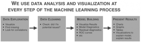
Data analysis and data visualization are critical at almost every part of the machine learning workflow.

So, to get started with ML (and to eventually master it) you need to be able to apply visualization and analysis.

In this post, I’ll show you some of the basic data analysis and visualization techniques you’ll need to know to build a machine learning model.

We’ll work on a toy problem, for simplicity and clarity

One note before we get started: the problem that we’ll work through is just linear regression and we’ll be using an easy-to-use, off-the-shelf dataset. It’s a “toy problem,” which is intentional. Whenever you try to learn a new skill, it is extremely helpful to isolate different details of that skill.

The skill that I really want you to focus on here is data visualization (as it applies to machine learning).

We’ll also be performing a little bit of data manipulation, but it will be in service of analyzing and visualizing the data. We won’t be doing any data manipulation to “clean” the data.

So just keep that in mind. We’re working on a very simplified problem. I’m removing or limiting several other parts of the ML workflow so we can strictly focus on preliminary visualization and analysis for machine learning.

Step 1: get the data

The first step almost of any analysis or model building effort is getting the data.

For this particular analysis, we’ll use a relatively “off the shelf” dataset that’s available in R within the MASS package.

data(Boston, package = "MASS")

The dataset contains data on median house price for houses in the Boston area. The variable that we’ll try to predict is the variable (median house price). The dataset has roughly a dozen other predictors that we’ll be investigating and using in our model.

This is a simplified “toy example” data doesn’t require much cleaning

As I already mentioned, the example we’ll be working through is a bit of a “toy” example, and as such, we’re working with a dataset that’s relatively “easy to use.” What I mean is that I’ve chosen this dataset because it’s easy to obtain and it doesn’t require much data cleaning.

However, keep in mind that in a typical business or industry setting, you’ll probably need to get your data from a database using SQL or possibly from a spreadsheet or other file.

Moreover, it’s very common for data to be “messy.” The data may have lots of missing values; variable names and class names that need to be changed; or other details that need to be altered.

Again, I’m intentionally leaving “data cleaning” out of this blog post for the sake of simplicity.

Just keep in mind that in many cases, you’ll have some data cleaning to do.

Step 2: basic data exploration

After getting the dataset, the next step in the model building workflow is almost always data visualization. Specifically, we’ll perform exploratory data analysis on the data to accomplish several tasks:

1. View data distributions
2. Identify skewed predictors
3. Identify outliers

Visualize data distributions

Let’s begin our data exploration by visualizing the data distributions of our variables.

We can start by visualizing the distribution of our target variable, .

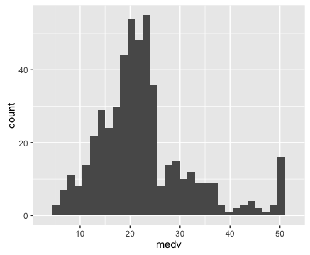
To do this, we’ll first use a basic histogram.

I strongly believe that the histogram is one of the “core visualization techniques” that every data scientists should master. If you want to be a great data scientist, and if you ultimately want to build machine learning models, then mastering the histogram is one of your “first steps.”

By “master”, I mean that you should be able to write this code “with your eyes closed.” A good data scientist should be able to write the code to create a histogram (or scatterplot, or line chart ….) from scratch, without any reference material and without “copying and pasting.” You should be able to write it from memory almost as fast as you can type.

One of the reasons that I believe the histogram is so important is because we use it frequently in this sort of exploratory data analysis. When we’re performing an analysis or building a model, it is extremely common to examine the distribution of a variable. Because it’s so common to do this, you should know this technique cold.

Here’s the code to create a histogram of our target variable .

############################
# VISUALIZE TARGET VARIABLE
############################

require(ggplot2)

#~~~~~~~~~~~
# histogram
#~~~~~~~~~~~

ggplot(data = Boston, aes(x = medv)) +
  geom_histogram()

2_data-analysis-for-ML_histogram-medv_2016-05-16

If you don’t really understand how this code works, I’d highly recommend that you read my blog post about how to create a histogram with ggplot2. That post explains how the histogram code works, step by step.

Let’s also create a density plot .

Here’s the exact code to create a density plot .

#~~~~~~~~~~~~~~
# density plot
#~~~~~~~~~~~~~~

ggplot(data = Boston, aes(x = medv)) +
  stat_density()

The density plot is essentially a variation of the histogram. The code to create a density plot is essentially identical to the code for a histogram, except that the second line is changed from to . Speaking in terms of ggplot2 syntax, we’re replacing the histogram geom with a statistical transformation.

3_data-analysis-for-ML_density-medv_2016-05-16

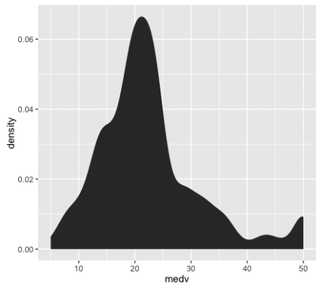
If you’ve been working with data visualization for a while, you might want to learn a little bit about the differences between histograms and density plots, and how we use them. This is more of an intermediate data visualization topic, but it’s relevant to this blog post on ‘data visualization for machine learning’, so I’ll mention it.

Between histograms and density plots, some people strongly prefer histograms. The primary reason for this is that histograms tend to “provide better information on the exact location of data” (which is good for detecting outliers). This is true in particular when you use a relatively larger number of histogram bins; a histogram with a sufficiently large number of bins can show you peaks and unusual data details a little better, because it doesn’t smooth that information away. (Density plots and histograms with a small number of bins can smooth that information out too much.) So, when we’re visualizing a single variable, the histogram might be the better option.

However, when we’re visualizing multiple variables at a time, density plots are easier to work with. If you attempt to plot several histograms at the same time by using a small multiple chart, it can be very difficult to select a single binwidth that properly displays all of your variables. Because of this, density plots are easier to work with when you’re visualizing multiple variables in a small multiple chart. Density plots show the general shape of the data and we don’t have to worry about choosing the number of bins.

Ok, so having plotted the distribution of our target variable, let’s examine the plots. We can immediately see a few important details:

1. It’s not perfectly normal.

This is one of the things we’re looking for when we visualize our data (particularly for linear regression). I’ll save a complete explanation of why we test for normality in linear regression and machine learning, but in brief, we are examining this because many machine learning techniques require normally distributed variables.

2. It appears that there may be a few minor outliers in the far right tail of the distribution. For the sake of simplicity, we’re not going to deal with those outliers here; we’ll be able to build a model (imperfect though it might be) without worrying about those outliers right now.

Keep in mind, however, that you’ll be looking for them when you plot your data, and in some cases, they may be problematic enough to warrant some action.

Now that we’ve examined our target variable, let’s look at the distributions of all of the variables in our dataset.

We’re going to visualize all of our predictors in a single chart, like this:

4_data-analysis-for-ML_variable-small-multiple_2016-05-16

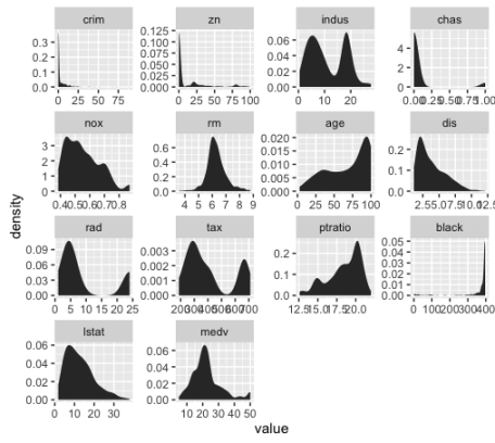
This is known as a small multiple chart (sometimes also called a “trellis chart”). Basically, the small multiple chart allows you to plot many charts in a grid format, side by side. It allows you to use the same basic graphic or chart to display different slices of a data set. In this case, we’ll use the small multiple to visualize different variables.

You might be tempted to visualize each predictor individually – one chart at a time – but that can get cumbersome and tedious very quickly. When you’re working with more than a couple of variables, the small multiple will save you lots of time. This is particularly true if you work with datasets with dozens, even hundreds of variables.

Although the small multiple is perfect for a task like this, we’ll have to do some minor data wrangling to use it.

Reshape the data for the small multiple chart

To use the small multiple design to visualize our variables, we’ll have to manipulate our data into shape.

Before we reshape the data, let’s take a look at the data as it currently exists:

head(Boston)

5_data-analysis-for-ML_head-boston-dataset_2016-05-16

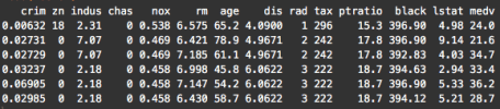
Notice that the variables are currently located as columns of the data frame. For example, the variable is the first column. This is how data is commonly formatted in a data frame; typical data frames have variables as columns, and data observations as rows. This format is commonly called “wide-format” data.

However, to create a “small multiple” to plot all of our variables, we need to reshape our data so that the variables are along the rows; we need to reshape our data into “long-format.’

To do this, we’re going to use the function from the package. This function will change the shape of the data from wide-format to long-format.

require(ggplot2)
require(reshape2)
melt.boston <- melt(Boston)
head(melt.boston)

6_data-analysis-for-ML_melt-boston-dataset_2016-05-16

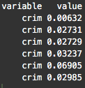
After using , notice that the variable (which had been a column) is now dispersed along the rows of our reshaped dataset, . In fact, if you examine the whole dataset, all of our dataset features are now along rows.

Now that we’ve melted our data into long-format, we’re going to use ggplot2 to create a small multiple chart. Specifically, we’ll use to implement the small-multiple design.

ggplot(data = melt.boston, aes(x = value)) +
  stat_density() +
  facet_wrap(~variable, scales = "free")

4_data-analysis-for-ML_variable-small-multiple_2016-05-16

So now that we’ve visualized the distributions of all of our variables, what are we looking for?

We’re looking primarily for a few things:

1. Outliers
2. Skewness
3. Other deviations from normality

Let’s examine skewness first (simply because that seems to be one of the primary issues with these features).

Just to refresh your memory, skewness is a measure of asymmetry of a data distribution.

You can immediately see that several of the variables are highly skewed .

In particular, , , , , and are highly skewed. Several of the others appear to have moderate skewness.

We’ll quickly confirm this by calculating the skewness:

#~~~~~~~~~~~~~~~~~~~~
# calculate skewness
#~~~~~~~~~~~~~~~~~~~~

require(e1071)
sapply(Boston, skewness)

7_data-analysis-for-ML_sapply-skewness-boston_2016-05-16

To be clear, skewness can be a bit of a slippery concept, but note that a skewness of zero indicates a symmetrical distribution. Ideally, we’re looking for variables with a skewness of zero.

Also, a very rough rule of thumb is if the absolute value of skewness is above 1, then the variable has high skewness.

Looking at these numbers, a few of the variables have relatively low skewness, including , , and (although is much more symmetrical).

Note: how we (normally) use this info

Part of the task of data exploration for ML is knowing what to do with the information uncovered in the data exploration process. That is, once you’ve identified potential problems and salient characteristics of your data, you need to be able to transform your data in ways that will make the machine learning algorithms work better. As I said previously, “data transformation” is a separate skill, and because we’re focusing on the pure “data exploration” process in this post, we won’t discussing data transformations. (Transformations are a big topic.)

Be aware, however, that in a common ML workflow, your learnings from EDA will serve as an input to the “data transformation” step of your workflow.

Recap

Let’s recap what we just did:

1. Plotted a histogram of our target variable using ggplot2
2. Reshaped our dataset using melt()
3. Plotted the variables using the small multiple design
4. Examined our variables for skewness and outliers

To be honest, this was actually an abbreviated list of things to do. We could also have looked at correlation, among other things.

This is more than enough to get you started though.

Tools that we leveraged.

By now, you should have some indication of what skills you need to know to get started with practical machine learning in R:

1. Learn ggplot2
– master basic techniques like the histogram and scatterplot
– learn how to facet your data in ggplot2 to perform multivariate data exploration

2. Learn basic data manipulation. I’ll suggest dplyr (which we didn’t really use here), and also reshape.

Want to see part 2?

In the next post, we’ll continue our use of data analysis in the ML workflow.

If you want to see part 2, sign up for the email list, and the next blog post will be delivered automatically to your inbox as soon as it’s published.

The post How to use data analysis for machine learning (example, part 1) appeared first on SHARP SIGHT LABS.

To leave a comment for the author, please follow the link and comment on their blog: r-bloggers – SHARP SIGHT LABS.

R-bloggers.com offers daily e-mail updates about R news and tutorials on topics such as: Data science, Big Data, R jobs, visualization (ggplot2, Boxplots, maps, animation), programming (RStudio, Sweave, LaTeX, SQL, Eclipse, git, hadoop, Web Scraping) statistics (regression, PCA, time series, trading) and more...


from R-bloggers http://ift.tt/1O2OMXR
via IFTTT

lunes, 23 de mayo de 2016

Evaluate the Performance of Machine Learning Algorithms in Python using Resampling

You need to know how well your algorithms perform on unseen data.

The best way to evaluate the performance of an algorithm would be to make predictions for new data to which you already know the answers. The second best way is to use clever techniques from statistics called resampling methods that allow you to make accurate estimates for how well your algorithm will perform on new data.

In this post you will discover how you can estimate the accuracy of your machine learning algorithms using resampling methods in Python and scikit-learn.

Let’s get started.

Evaluate the Performance of Machine Learning Algorithms in Python using Resampling

Evaluate the Performance of Machine Learning Algorithms in Python using Resampling
Photo by Doug Waldron, some rights reserved.

About The Recipes

Resampling methods are demonstrated in this post using small code recipes in Python.

Each recipe is designed to be standalone so that you can copy-and-paste it into your project and use it immediately.

The Pima Indians onset of diabetes dataset is used in each recipe. This is a binary classification problem where all of the input variables are numeric. In each recipe it is downloaded directly from the UCI Machine Learning repository. You can replace it with your own dataset as needed.

Evaluate Your Machine Learning Algorithms

Why can’t you train your machine learning algorithm on your dataset and use predictions from this same dataset to evaluate machine learning algorithms?

The simple answer is overfitting.

Imagine an algorithm that remembers every observation it is shown. If you evaluated your machine learning algorithm on the same dataset used to train the algorithm, then an algorithm like this would have a perfect score on the training dataset. But the predictions it made on new data would be terrible.

We must evaluate our machine learning algorithms on data that is not used to train the algorithm.

The evaluation is an estimate that we can use to talk about how well we think the algorithm may actually do in practice. It is not a guarantee of performance.

Once we estimate the performance of our algorithm, we can then re-train the final algorithm on the entire training dataset and get it ready for operational use.

Next up we are going to look at four different techniques that we can use to split up our training dataset and create useful estimates of performance for our machine learning algorithms:

  1. Train and Test Sets.
  2. K-fold Cross Validation.
  3. Leave One Out Cross Validation.
  4. Repeated Random Test-Train Splits.

We will start with the simplest method called Train and Test Sets.

1. Split into Train and Test Sets

The simplest method that we can use to evaluate the performance of a machine learning algorithm is to use different training and testing datasets.

We can take our original dataset, split it into two parts. Train the algorithm on the first part, make predictions on the second part and evaluate the predictions against the expected results.

The size of the split can depend on the size and specifics of your dataset, although it is common to use 67% of the data for training and the remaining 33% for testing.

This algorithm evaluation technique is very fast. It is ideal for large datasets (millions of records) where there is strong evidence that both splits of the data are representative of the underlying problem. Because of the speed, it is useful to use this approach when the algorithm you are investigating is slow to train.

A downside of this technique is that it can have a high variance. This means that differences in the training and test dataset can result in meaningful differences in the estimate of accuracy.

In the example below we split the data Pima Indians dataset into 67%/33% split for training and test and evaluate the accuracy of a Logistic Regression model.

# Evaluate using a train and a test set
import pandas
from sklearn import cross_validation
from sklearn.linear_model import LogisticRegression
url = "http://ift.tt/1Ogiw3p;
names = ['preg', 'plas', 'pres', 'skin', 'test', 'mass', 'pedi', 'age', 'class']
dataframe = pandas.read_csv(url, names=names)
array = dataframe.values
X = array[:,0:8]
Y = array[:,8]
test_size = 0.33
seed = 7
X_train, X_test, Y_train, Y_test = cross_validation.train_test_split(X, Y, test_size=test_size, random_state=seed)
model = LogisticRegression()
model.fit(X_train, Y_train)
result = model.score(X_test, Y_test)
print("Accuracy: %.3f%%") % (result*100.0)

We can see that the estimated accuracy for the model was approximately 75%. Note that in addition to specifying the size of the split, we also specify the random seed. Because the split of the data is random, we want to ensure that the results are reproducible. By specifying the random seed we ensure that we get the same random numbers each time we run the code.

This is important if we want to compare this result to the estimated accuracy of another machine learning algorithm or the same algorithm with a different configuration. To ensure the comparison was apples-for-apples, we must ensure that they are trained and tested on the same data.

Accuracy: 75.591%

2. K-fold Cross Validation

Cross validation is an approach that you can use to estimate the performance of a machine learning algorithm with less variance than a single train-test set split.

It works by splitting the dataset into k-parts (e.g. k=5 or k=10). Each split of the data is called a fold. The algorithm is trained on k-1 folds with one held back and tested on the held back fold. This is repeated so that each fold of the dataset is given a chance to be the held back test set.

After running cross validation you end up with k different performance scores that you can summarize using a mean and a standard deviation.

The result is a more reliable estimate of the performance of the algorithm on new data given your test data. It is more accurate because the algorithm is trained and evaluated multiple times on different data.

The choice of k must allow the size of each test partition to be large enough to be a reasonable sample of the problem, whilst allowing enough repetitions of the train-test evaluation of the algorithm to provide a fair estimate of the algorithms performance on unseen data. For modest sized datasets in the thousands or tens of thousands of records, k values of 3, 5 and 10 are common.

In the example below we use 10-fold cross validation.

# Evaluate using Cross Validation
import pandas
from sklearn import cross_validation
from sklearn.linear_model import LogisticRegression
url = "http://ift.tt/1Ogiw3p;
names = ['preg', 'plas', 'pres', 'skin', 'test', 'mass', 'pedi', 'age', 'class']
dataframe = pandas.read_csv(url, names=names)
array = dataframe.values
X = array[:,0:8]
Y = array[:,8]
num_folds = 10
num_instances = len(X)
seed = 7
kfold = cross_validation.KFold(n=num_instances, n_folds=num_folds, random_state=seed)
model = LogisticRegression()
results = cross_validation.cross_val_score(model, X, Y, cv=kfold)
print("Accuracy: %.3f%% (%.3f%%)") % (results.mean()*100.0, results.std()*100.0)

You can see that we report both the mean and the standard deviation of the performance measure. When summarizing performance measures, it is a good practice to summarize the distribution of the measures, in this case assuming a Gaussian distribution of performance (a very reasonable assumption) and recording the mean and standard deviation.

Accuracy: 76.951% (4.841%)

3. Leave One Out Cross Validation

You can configure cross validation so that the size of the fold is 1 (k is set to the number of observations in your dataset). This variation of cross validation is called leave-one-out cross validation.

The result is a large number of performance measures that can be summarized in an effort to give a more reasonable estimate of the accuracy of your model on unseen data. A downside is that it can be a computationally more expensive procedure than k-fold cross validation.

In the example below we use leave-one-out cross validation.

# Evaluate using Leave One Out Cross Validation
import pandas
from sklearn import cross_validation
from sklearn.linear_model import LogisticRegression
url = "http://ift.tt/1Ogiw3p;
names = ['preg', 'plas', 'pres', 'skin', 'test', 'mass', 'pedi', 'age', 'class']
dataframe = pandas.read_csv(url, names=names)
array = dataframe.values
X = array[:,0:8]
Y = array[:,8]
num_folds = 10
num_instances = len(X)
loocv = cross_validation.LeaveOneOut(n=num_instances)
model = LogisticRegression()
results = cross_validation.cross_val_score(model, X, Y, cv=loocv)
print("Accuracy: %.3f%% (%.3f%%)") % (results.mean()*100.0, results.std()*100.0)

You can see in the standard deviation that the score has more variance than the k-fold cross validation results described above.

Accuracy: 76.823% (42.196%)

4. Repeated Random Test-Train Splits

Another variation on k-fold cross validation is to create a random split of the data like the train/test split described above, but repeat the process of splitting and evaluation of the algorithm multiple times, like cross validation.

This has the speed of using a train/test split and the reduction in variance in the estimated performance of k-fold cross validation. You can also repeat the process many more times as need. A down side is that repetitions may include much of the same data in the train or the test split from run to run, introducing redundancy into the evaluation.

The example below splits the data into a 67%/33% train/test split and repeats the process 10 times.

# Evaluate using Shuffle Split Cross Validation
import pandas
from sklearn import cross_validation
from sklearn.linear_model import LogisticRegression
url = "http://ift.tt/1Ogiw3p;
names = ['preg', 'plas', 'pres', 'skin', 'test', 'mass', 'pedi', 'age', 'class']
dataframe = pandas.read_csv(url, names=names)
array = dataframe.values
X = array[:,0:8]
Y = array[:,8]
num_samples = 10
test_size = 0.33
num_instances = len(X)
seed = 7
kfold = cross_validation.ShuffleSplit(n=num_instances, n_iter=num_samples, test_size=test_size, random_state=seed)
model = LogisticRegression()
results = cross_validation.cross_val_score(model, X, Y, cv=kfold)
print("Accuracy: %.3f%% (%.3f%%)") % (results.mean()*100.0, results.std()*100.0)

We can see that the distribution of the performance measure is on par with k-fold cross validation above.

Accuracy: 76.496% (1.698%)

What Techniques to Use When

  • Generally k-fold cross validation is the gold-standard for evaluating the performance of a machine learning algorithm on unseen data with k set to 3, 5, or 10.
  • Using a train/test split is good for speed when using a slow algorithm and produces performance estimates with lower bias when using large datasets.
  • Techniques like leave-one-out cross validation and repeated random splits can be useful intermediates when trying to balance variance in the estimated performance, model training speed and dataset size.

The best advice is to experiment and find a technique for your problem that is fast and produces reasonable estimates of performance that you can use to make decisions. If in doubt, use 10-fold cross validation.

Your Guide to Machine Learning with Scikit-Learn

Python Mini-CoursePython and scikit-learn are the rising platform among professional data scientists for applied machine learning.

PDF and Email Course.

FREE 14-Day Mini-Course in
Machine Learning with Python and scikit-learn

Download Your FREE Mini-Course >>


 Download your PDF containing all 14 lessons.

Get your daily lesson via email with tips and tricks.


Summary

In this post you discovered statistical techniques that you can use to estimate the performance of your machine learning algorithms, called resampling.

Specifically, you learned about:

  1. Train and Test Sets.
  2. Cross Validation.
  3. Leave One Out Cross Validation.
  4. Repeated Random Test-Train Splits.

Do you have any questions about resampling methods or this post? Ask your question in the comments and I will do my best to answer it.

Can You Step-Through Machine Learning Projects 
in Python with scikit-learn and Pandas?

Machine Learning Mastery with PythonDiscover how to confidently step-through machine learning projects end-to-end in Python with scikit-learn in the new Ebook: 

Machine Learning Mastery with Python

Take the next step with 16 self-study lessons covering data preparation, feature selection, ensembles and more.

Includes 3 end-to-end projects and a project template to tie it all together.

Ideal for beginners and intermediate levels.

Apply Machine Learning Like A Professional With Python

The post Evaluate the Performance of Machine Learning Algorithms in Python using Resampling appeared first on Machine Learning Mastery.


from Machine Learning Mastery http://ift.tt/1TCp10O
via IFTTT

viernes, 20 de mayo de 2016

5 Machine Learning Projects You Can No Longer Overlook

We all know the big machine learning projects out there: Scikit-learn, TensorFlow, Theano, etc. But what about the smaller niche projects that are actively developed, providing useful services to users? Here are 5 such projects.

The popular machine learning projects, in general, are popular because they either provide a wide range of needed services or they were the first (or possibly best) to provide a particular niche service to users. These popular projects include Scikit-learn, TensorFlow, Theano, MXNet (maybe?), Weka (formerly), and so on. Depending on the particular ecosystem(s) you work in, and on your machine learning goals, the projects which you consider popular may differ slightly; however, they all share the similarity that they provide services to a large base of users.

But there are all sorts of smaller machine learning projects out there that people are building and using: pipelines, wrappers, high-level APIs, cleaners, etc. They provide both niche and flexible services, usually for smaller numbers of users, for all sorts of reasons. This post will present 5 such smaller projects for readers to familiarize themselves with.

I'm not necessarily suggesting you go out and try all (or any) of these; if there is some particular requirement you are looking to fill which you happen to find a corresponding tool for in this list, then by all means give it a try. The real value here, however, at least in my view, is checking out what the projects offer, how they are implemented, and what others are building to fit into their ecosystems. You might get some good ideas of where to take your own projects. But best case: something here fills a need perfectly and you solve a problem, thanks to the work the developers listed herein are doing.

There is no real criteria for these items, I'm sorry to report. They are simply a collection of interesting projects I have noted over the past few months and thought were promising enough to share with readers. Also note that I am firmly invested in the Python ecosystem, and so these tools have been discovered accordingly. I don't have any bias against any of the projects that R or C++ or any other particular environment has to offer (and may discover and share such projects in future posts); this list came together generically, however, based on my internet wanderings as I searched for useful tools.

So here they are: 5 machine learning projects you should definitely have a look at, in no particular order (but numbered like they are in order, because I like numbering things):

1. Deepy

Deepy is an extensible deep learning framework based on Theano. It provides a clean, high-level interface for components such as LSTMs, Batch Normalization, and Auto Encoders. Deepy clearly aims for simplicity, and its documentation and examples aim for the same. It also has a sister project, which uses Deepy to implement Deep Recurrent Attentive Writer (DRAW) generative models.

For an example of Deepy's simplicity and cleanliness, here's an example of a multi-layer model with dropout, from the project's Github:

# A multi-layer model with dropout for MNIST task.
from deepy import *

model = NeuralClassifier(input_dim=28*28)
model.stack(Dense(256, 'relu'),
            Dropout(0.2),
            Dense(256, 'relu'),
            Dropout(0.2),
            Dense(10, 'linear'),
            Softmax())

trainer = MomentumTrainer(model)

annealer = LearningRateAnnealer(trainer)

mnist = MiniBatches(MnistDataset(), batch_size=20)

trainer.run(mnist, controllers=[annealer])

You may have even heard of Deepy already; its Github repo has 305 stars and has been forked 51 times, as of this writing. The project is a decent exemplar of high-level deep learning APIs and wrappers that are becoming widespread (or seem to be). Deepy is authored by Raphael Shu.

2. MLxtend

Sebastian Raschka has put together MLxtend, something he is quick to point out is a work in progress, but is also something which attempts to tick a number of different boxes. MLxtend is a collection of useful tools and extensions for machine learning tasks.

MLxtend

Sebastian shared the following with me, regarding the project, how it came to be, and its goals:

Essentially, it's just a collection of useful tools and reference implementations related to ML and data science in general. Why did I come up with it? There are a couple of reasons:

  1. Implementations of algorithms that I couldn't find anywhere else (e.g., the Sequential Feature Selection algorithms, the Majority Voting Classifier, the Stacking estimators, plotting decision regions, ...)
  2. Implementations for teaching purposes (logistic regression, softmax regression, multi-layer perceptron, PCA, kernel PCA...); these impl. focus on code readability rather than pure efficiency
  3. Wrappers for convenience: tensorflow softmax regression and multi-layer perceptrons, column-wise standardization for pandas data frames

This is essentially a library of commonly-used general machine learning functions that Sebastian has written and frequently uses. Additionally, Sebastian really likes to code, and thought that if he were to offer this "zoo" of different things (as he refers to it) up to others that he may keep the code "tidier" than usual.

Many of the implemented functions share similarities with scikit-learn's API, but future addition functionality will not necessarily be restricted by this. The big takeaway here: Sebastian promises that there is much more to come... so stay tuned. There's a good chance that any feature or novel algorithm that Sebastian plays with will end up being packaged in MLxtend.

3. datacleaner

datacleaner is the work of researcher Randal Olson, who is also responsible for the fantastic TPOT machine learning pipeline project. Olson bills Data Cleaner as a "Python tool that automatically cleans data sets and readies them for analysis." He is quick to declare that it is not magic, but also points out what it can do:

What datacleaner will do is save you a ton of time encoding and cleaning your data once it's already in a format that pandas DataFrames can handle.

datacleaner is a work in progress, but is currently capable of handling the following regular (and time-consuming) data cleaning operations: optionally drops rows with missing values; replaces missing values with either mode or median, on a column by column basis; encodes non-numerical variables with numerical equivalents. Randal tells us that he is looking for contributors, especially from those with more ideas on what data cleaning operations datacleaner could perform in an automated fashion.

Randal has an attention to detail that anyone who reads his blog or his Github repos already knows, and the concise documentation for this project is no exception. I have been using datacleaner recently, and so far it delivers on its promises.

4. auto-sklearn

auto-sklearn is automated machine learning for the Scikit-learn environment.

auto-sklearn frees a machine learning user from algorithm selection and hyperparameter tuning. It leverages recent advantages in Bayesian optimization, meta-learning and ensemble construction. Learn more about the technology behind auto-sklearn by reading this paper published at the NIPS 2015.

auto-sklearn

Its documentation is quite thorough, and the repo includes a few concise examples. I have, admittedly, not used it yet, but many others have; it has collected nearly 400 stars on Github. Given my propensity for Scikit-learn, I imagine I will try this out in the near future.

auto-sklearn is developed mainly by the Machine Learning for Automated Algorithm Design group at the University of Freiburg.

5. Deep Mining

Deep Mining is a machine learning pipeline auto-tuner, coming to us from Sebastien Dubois of the CSAIL lab at MIT. From the repo:

This software will test iteratively, and smartly, some hyperparameter sets in order to find as quickly as possible the best ones to achieve the best classification accuracy that a pipeline can offer.

Deep Mining

Deep Mining does not seem to be a well-known project, given its relatively modest number of repo stars; however, given that it comes out of CSAIL, and has development activity within the past month, it may be worth benchmarking this against other similar automated pipeline tools. It comes with a few examples, and its usage seems to be straightforward.

More on the methods used:

The folder GCP-HPO contains all the code implementing the Gaussian Copula Process (GCP) and a hyperparameter optimization (HPO) technique based on it. Gaussian Copula Process can be seen as an improved version of the Gaussian Process, that does not assume a Gaussian prior for the marginal distributions but lies on a more complex prior. This new technique is proved to outperform GP-based hyperparameter optimization, which is already far better than the randomized search.

A paper on the GCP approach is forthcoming.

Related:


from KDnuggets http://ift.tt/1OPb27O
via IFTTT