Dogra, Shaillay K., "Normalization." From QSARWorld--A Strand Life Sciences Web Resource.
http://www.qsarworld.com/qsar-statistics-normalization.php
Normalization
Most of the computed descriptors differ in the scales in which their values lie. One may need to normalize them before proceeding with further statistical analysis. This mostly depends on the subsequent Machine Learning algorithms that one wants to run on the data.
Algorithms like Decision Trees, Regression Forest, Decision Forest and Naïve Bayes do not require normalized data as input. For Linear Regression, normalization is a recommended step. For Neural Networks – classification or regression, Support Vector Machines – classification or regression, normalization of data is required.
In context of cheminformatics, a standard way to normalize data is by mean shifting and auto-scaling. This makes the mean of a thus transformed descriptor column as 0 and the standard deviation as 1.
Mean Shifting
Most of the computed descriptors differ in the scales in which their values lie. One may thus want to normalize them before proceeding with further statistical analysis. As part of normalization, each value for a given descriptor (all values in a column) is adjusted or shifted by the mean value. As a result, the new mean value becomes 0. This happens for all the descriptors and they thus now have the same mean value 0. Hence, mean, as a measure of central location of the distribution of values, for all the descriptors, is now the same. However, the 'spread' or the 'variation' in the data, about the mean, is still the same as in the original data. This can now be taken care of by scaling the values with the standard deviation.
This is best illustrated with an example. Consider these numbers: 1, 2, 3, 4, and 5. The total of these numbers is 15 and the mean is 3. Adjusting each value by the mean value gives the transformed numbers as: -2, -1, 0, 1, and 2. The new total is 0 and thus the new mean is 0. However, note that the standard deviation is still the same as original (√2). This can now be taken care of by scaling the values with standard deviation in order to make the new standard deviation as 1.
Autoscaling
For a given set of values, the standard deviation can be made to be unit by scaling (dividing) all the values by the original standard deviation. This is a standard step in normalization of data.
Say, the values are - 1, 2, 3, 4 and 5. The standard deviation is √2. Now, dividing each value by the standard deviation gives us the transformed data as - 1/√2, √2, 3/√2, 2√2 and 5/√2. The new standard deviation for this set of values is 1.
(The above principle is better demonstrated algebraically).
A value x belonging to a distribution with mean 'x_mean' and standard deviation 's' can be transformed to a standard score, or z-score, in the following manner:
z = (x - x_mean)/s
The mean of standard scores is zero. When values are standardized, the units in which they are expressed are equal to the standard deviation, s. For the standardized scores, the standard deviation becomes 1. (Variance is also 1). The interpretation of the standard-score of a given value is in terms of the number of standard deviations the value is above or below the mean (of the distribution of standardized scores).
So, the standardization of a set of values involves two steps. First, the mean is subtracted from every value, which shifts the central location of the distribution to 0. Then the thus mean-shifted values are divided by the standard deviation, s. This now makes the standard deviation as 1.
miércoles, 14 de octubre de 2009
Some Interesting Links about CUDA Programming
Getting started with CUDA
CUDA Tutorial
HPCWire.com
multicoreinfo.com
Videos
Scalable Parallel Programming with CUDA on Manycore GPUs
Stanford University Computer Systems Colloquium (EE 380).
John Nickolls - NVIDIA
CUDA Tutorial
HPCWire.com
multicoreinfo.com
Videos
Scalable Parallel Programming with CUDA on Manycore GPUs
Stanford University Computer Systems Colloquium (EE 380).
John Nickolls - NVIDIA
Model Applicability
Dogra, Shaillay K., "Model Applicability" From QSARWorld--A Strand Life Sciences Web Resource.
http://www.qsarworld.com/insilico-chemistry-model-applicability.php
When using a model for predicting the value(s) for some unknown compound(s), assessment of the applicability of the model, in context of the compound(s) under study, is necessary. This can be assessed with different approaches, all of which in some sense try to assess whether the structure-, chemical-, or descriptor-based properties of the ‘unknown’ compound lie in similar ‘space’ as those for the compounds that were part of the training set used for building the model. This is an issue because the basic assumption of QSAR modeling is that similar compounds have similar activity/property and hence, given an unknown compound, we shall be able to predict its activity/property with confidence if it is ‘similar’ to the compounds that were used for building the model.
Whether the compound(s) under study is ‘similar’ to the training set compounds can be assessed in various ways:
1) Structure-based similarity: Tanimoto coefficient values, obtained by comparing MACCS fingerprints, can be used to assess structural similarity. If any of the training set compound has a Tanimoto coefficient value > 0.85 when compared against the compound under study, the same can be taken as an indication of high structural similarity and it can be believed that the given model is applicable for this case.
2)Descriptor-based similarity: Similarity of the compound under study against the compounds in the training set can also be estimated by computing the distances (Euclidean) of the descriptors, that were used in training the model, between the unknown compound(s) and the training set compounds. This distance should lie between 0 to ∞ and possibly, the lesser the distance the better it is.
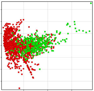
3) Chemical Space: Comparing the ‘chemical space’ of the ‘unknown’ compounds against the compounds in the training set (used for building the model) can be another way to assess model applicability. What can be done here is to run a Principal Components Analysis (PCA) on the descriptors used in the model, for both the training set and the ‘unknown’ compounds, and then launch a plot on the first two components. In the figure below, the training set compounds are shown in red while the ‘unknown’ compounds, for which the predictions need to be made, are depicted in green. Thus, at a glance it can be visualized if the ‘unknown’ compounds belong to the same distribution or ‘space’ as the ones used for deriving the model (and decide for or against using the given model).
4) Statistical Measures: The model can anyway be used for predicting the values for the ‘unknown’ compounds. The predicted values usually also have a measure of statistical significance associated with them.
In case of regression models (prediction of a continuous value), this measure is in terms of standard error. A simple interpretation of the standard error is that, according to the model, the predicted value lies in an interval bound by +/- standard error with a 95% confidence. Say, the predicted value is x and the associated standard error is y, then the value is estimated to lie in x-y to x+y interval with a 95% confidence. (This however does not imply that there exists some interval wherein the confidence could be 100%).
In case of classification models (prediction of a categorical value), the statistical significance is in terms of confidence measure. This lies in a 0-1 scale and can be interpreted as the % confidence that the underlying algorithm (in the model) has when it is predicting some given compound to belong to a particular class. Say, if an ‘unknown’ compound is called by the model to belong to a particular class, and the model associates a confidence measure of 0.90 with that prediction, this implies that the algorithm is 90% confident about making this prediction. In other words, statistically, in the long run, when the algorithm makes large enough such predictions, 90% of them would turn out to be correct.
http://www.qsarworld.com/insilico-chemistry-model-applicability.php
When using a model for predicting the value(s) for some unknown compound(s), assessment of the applicability of the model, in context of the compound(s) under study, is necessary. This can be assessed with different approaches, all of which in some sense try to assess whether the structure-, chemical-, or descriptor-based properties of the ‘unknown’ compound lie in similar ‘space’ as those for the compounds that were part of the training set used for building the model. This is an issue because the basic assumption of QSAR modeling is that similar compounds have similar activity/property and hence, given an unknown compound, we shall be able to predict its activity/property with confidence if it is ‘similar’ to the compounds that were used for building the model.
Whether the compound(s) under study is ‘similar’ to the training set compounds can be assessed in various ways:
1) Structure-based similarity: Tanimoto coefficient values, obtained by comparing MACCS fingerprints, can be used to assess structural similarity. If any of the training set compound has a Tanimoto coefficient value > 0.85 when compared against the compound under study, the same can be taken as an indication of high structural similarity and it can be believed that the given model is applicable for this case.
2)Descriptor-based similarity: Similarity of the compound under study against the compounds in the training set can also be estimated by computing the distances (Euclidean) of the descriptors, that were used in training the model, between the unknown compound(s) and the training set compounds. This distance should lie between 0 to ∞ and possibly, the lesser the distance the better it is.
3) Chemical Space: Comparing the ‘chemical space’ of the ‘unknown’ compounds against the compounds in the training set (used for building the model) can be another way to assess model applicability. What can be done here is to run a Principal Components Analysis (PCA) on the descriptors used in the model, for both the training set and the ‘unknown’ compounds, and then launch a plot on the first two components. In the figure below, the training set compounds are shown in red while the ‘unknown’ compounds, for which the predictions need to be made, are depicted in green. Thus, at a glance it can be visualized if the ‘unknown’ compounds belong to the same distribution or ‘space’ as the ones used for deriving the model (and decide for or against using the given model).

4) Statistical Measures: The model can anyway be used for predicting the values for the ‘unknown’ compounds. The predicted values usually also have a measure of statistical significance associated with them.
In case of regression models (prediction of a continuous value), this measure is in terms of standard error. A simple interpretation of the standard error is that, according to the model, the predicted value lies in an interval bound by +/- standard error with a 95% confidence. Say, the predicted value is x and the associated standard error is y, then the value is estimated to lie in x-y to x+y interval with a 95% confidence. (This however does not imply that there exists some interval wherein the confidence could be 100%).
In case of classification models (prediction of a categorical value), the statistical significance is in terms of confidence measure. This lies in a 0-1 scale and can be interpreted as the % confidence that the underlying algorithm (in the model) has when it is predicting some given compound to belong to a particular class. Say, if an ‘unknown’ compound is called by the model to belong to a particular class, and the model associates a confidence measure of 0.90 with that prediction, this implies that the algorithm is 90% confident about making this prediction. In other words, statistically, in the long run, when the algorithm makes large enough such predictions, 90% of them would turn out to be correct.
Suscribirse a:
Entradas (Atom)